PVA Lab
Name: Kyle Collins
Lab Partner: Parker Fairchild
Date: 2 October 2014
Purpose: The purpose of this lab is to use various data collection methods such as a ticker-tape timer and video recording in conjunction with a stopwatch to find the five kinematic quantities of a cart in motion down an inclined plane.
Theory: The PVA lab focused on the five basic kinematic quantities: initital velocity, final velocity, distance, acceleration, and time. Initial velocity and final velocity can both be described as the displacement of the object divided by the time. Distance is calculated by measuring the interval with a tool such as a meterstick. Time is calculated by using a stopwatch.
Experimental Technique: First, the angle that the cart would be traveling down was set at five degrees.

Close-Up of Angle Indicator
|

Full View of Track
|
Red tape was placed on the track, with the leading edges of the pieces at 90cm and 40cm, giving a distance of 50 cm for the cart to travel. Affixed to the cart was a red indicator that would facilitate the timing of the cart.

Tape at 90cm
|

Tape at 40cm
|

Red Pointer/Indicator Affixed to Cart
The first method involved timing the cart with a stopwatch as it passed between the tape intervals to calculate the total time. Then, slow-motion video recorded at thirty frames per second was used to calculate initial and final velocity by finding the distance traveled in the time span of one video frame. The distance was measured using a meterstick attached to the side of the track. After all the data had been collected using the first method, a ticker-tape timer was set up, which produced dots to be used for a position vs time graph.
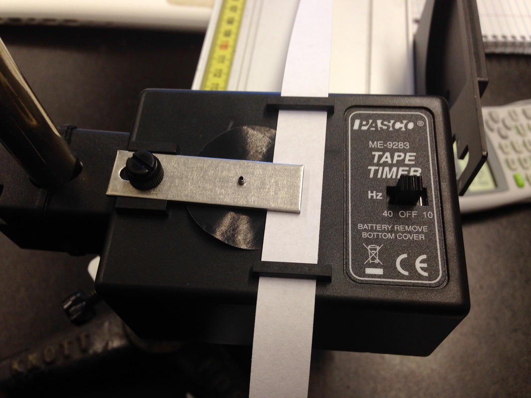
Ticker-Tape Timer, Main Unit
|

Ticker-Tape Attached to Cart
|
Data And Analysis
The first method used was using the stopwatch and video recording to produce the five kinematic quantities. The time the cart took to travel between the 50cm tape interval was .54 seconds. This was averaged from three runs. The video recording software used recorded at thirty frames per second, and so the time interval used in the calculation of velocity was .033s. Using the video recording software and the formulas for initial velocity and final velocity, velocities of 75.8cm/s and 121.2cm/s were produced, respectively.
The first method used was using the stopwatch and video recording to produce the five kinematic quantities. The time the cart took to travel between the 50cm tape interval was .54 seconds. This was averaged from three runs. The video recording software used recorded at thirty frames per second, and so the time interval used in the calculation of velocity was .033s. Using the video recording software and the formulas for initial velocity and final velocity, velocities of 75.8cm/s and 121.2cm/s were produced, respectively.

|

|

|

|

|

|
Next, acceleration was calculated by using the velocities above and dividing their difference by the total time, thus giving an average acceleration of 84.07cm/s/s. Note that the acceleration here is not constant, and is changing from instant to instant.


The complete equations, diagram, and math can be seen in the picture below:
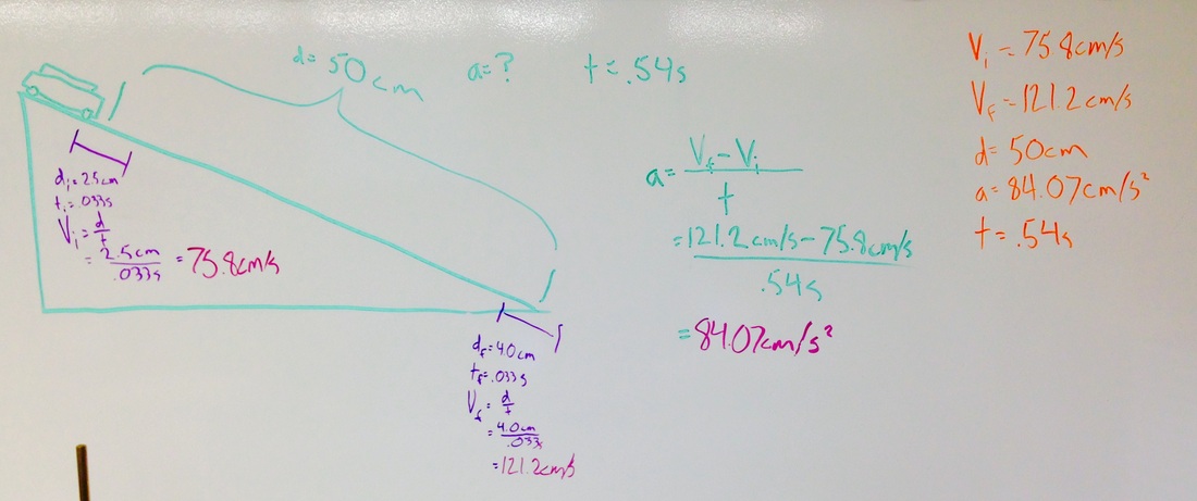
Complete Diagram
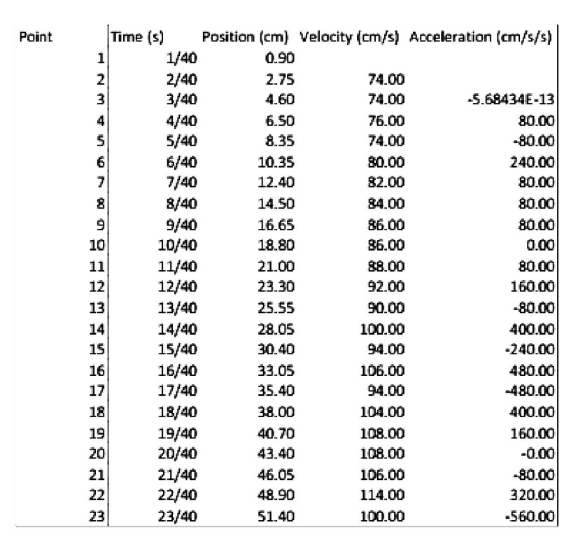
After completing the initial phase with the kinematic equations, using a ticker-tape timer to create position vs time graphs was the next step. The ticker-tape timer was set to tick at 40hz, and the cart was run down the track. The distances were then recorded and plotted as a function of time in a spreadsheet to create a position vs time graph. As it didn't take the cart one full second to move down the ramp, there were only twenty-three dots produced. To create the velocity vs time graph, the formula for velocity and position data from the table were used (below left). In this case, position is the same variable as distance, d. Finally, an acceleration vs time graph was created using the formula for acceleration and velocity data from the table (below right).

|

|
Below is the data table with all calculated numbers as well as various graphs.

|


|
In the position vs time graph, there is a very strong correlation between data points, and there is an r-value of .9961, indicating that correlation. The velocity vs time graph has a moderate correlation, and has a lower r-value of only .8972. Lastly is the acceleration vs time graph, which has almost no correlation, with a very low r-value of .0171. Both the position vs time graph and the velocity vs time graph had values that very closely related to the five kinematic quantities derived using the stopwatch and video software. For example, the initial and final velocities were the same, and the overall time is nearly the same. There is an interesting trend in the graphs, however. While the position graph is fairly straight, there is a little variation in the velocity graph, and the acceleration graph is very varied. This is because the graphs and points on them are derived by dividing the difference of the terms before them by time (ex. difference in position divided by time gives velocity). This division causes slight variations in the graph to become more exaggerated as the trend continues.
There is also a fair amount of error involved in this method. For example, a stopwatch is not the most precise measuring instrument, and there was certainly reaction time error present when using it. In the video we used to calculate initial and final velocities, there was a fair amount of blurriness, making it difficult to judge where the cart actually was. Friction was also not accounted for in the equations, but was present, making the numbers inaccurate. In measuring distance on the ticker-tape, the meterstick only gave a certain amount of precision and there was estimation error present.
Conclusion
The goals of this experiment were to use kinematic equations and various technological methods to predict motion in the real world. The results were similar to what was expected to occur. That being said, error was definitely present, and so while the answers may have been precise, they were probably not accurate. It likely stemmed from improper measuring techniques, as well as inconsistencies in the technology used. Were the experiment to be repeated, improvements would include more precise measuring tools, such as more advanced video software, and simple methods to reduce error, such as merely double-checking measurements. As a whole, this was a successful experiment.
